![]()
Introductory Statistics: Learning Objectives 4, 5, 6, 7
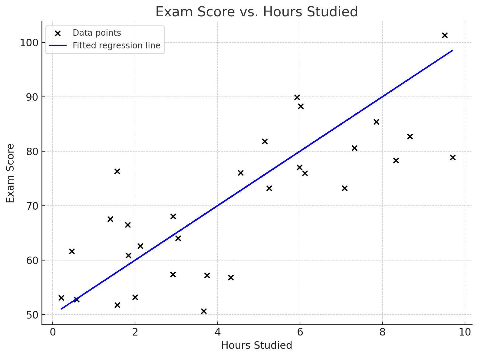
Question 1: Below is a scatterplot showing the relationship between the number of hours studied (x-axis) and exam score (y-axis) for 30 students. A simple linear regression line has been fit to the data and is shown in blue.
- Estimate the value of the intercept $\beta_0$, and provide an interpretation for this estimate.
- Estimate the value of the slope parameter $\beta_1$, and provide an interpretation for this estimate.
- Which of the following statements could be true concerning student's exam scores and number of hours studied?
- i. The proportion of explained variation is 0.64 and the correlation is 0.8.
- ii. The proportion of explained variation is 0.8 and the correlation is 0.64.
- iii. The proportion of explained variation is -0.64 and the correlation is 0.8.
- iv. The proportion of explained variation is 0.64 and the correlation is -0.8.
a) The intercept is the value on the y-axis where the line crosses (i.e., where x=0).
b) The slope is the "rise over run". Pick two points on the line and calculate the change in y divided by the change in x.
c) Remember that the proportion of explained variation is $R^2$, and the correlation is $r$. The relationship is $R^2 = r^2$. Also, consider the direction of the relationship shown in the plot.
- The intercept $\beta_0$ is approximately 50. This is the predicted exam score for a student who studied for 0 hours.
- The slope $\beta_1$ is approximately 5. For each additional hour a student studies, their exam score is predicted to increase by 5 points.
- i. The proportion of explained variation is 0.64 and the correlation is 0.8.
a) Intercept: The intercept is the value of Y when X is 0. Looking at the graph, the blue line crosses the y-axis at an exam score of 50. This means the model predicts a score of 50 for a student who did not study at all.
b) Slope: The slope is the change in Y for a one-unit change in X. Let's pick two points on the line to estimate it. The y-intercept is (0, 50). Another point on the line appears to be at (10 hours, 100 score). $$ \text{Slope} = \frac{\text{change in Y}}{\text{change in X}} = \frac{100 - 50}{10 - 0} = \frac{50}{10} = 5 $$ This means that for each additional hour of studying, the model predicts a 5-point increase in the exam score.
c) Proportion of Variation and Correlation: The "proportion of explained variation" is the coefficient of determination, $R^2$. The correlation is $r$. The relationship is $R^2 = r^2$.
- The scatterplot shows a positive relationship (as hours studied increases, score increases), so the correlation $r$ must be positive. This eliminates option (iv).
- The proportion of explained variation, $R^2$, cannot be negative. This eliminates option (iii).
- We now compare (i) and (ii). In (i), $r=0.8$ and $R^2=0.64$. This is consistent, since $0.8^2 = 0.64$. In (ii), $r=0.64$ and $R^2=0.8$. This is inconsistent, since $0.64^2 \neq 0.8$.
Question 2: You are reading a paper that compares depressive symptoms between men and women using Beck Depression Inventory (BDI) Score. The authors report the following data:
| Female (Mean $\pm$ SD) | Male (Mean $\pm$ SD) | |
|---|---|---|
| BDI Score | 11.98 $\pm$ 9.68 | 9.00 $\pm$ 7.93 |
- Let $M$ be an indicator variable such that $M=1$ indicates a male and $M=0$ indicates a female. The authors fit the following simple linear regression model to test for a difference in mean BDI score between men and women: \[ E[BDI] = \beta_0 + \beta_1 \times M\] Which of the following is the fitted regression equation based on the observed data?
- i. $E[BDI] = 11.98 + 9.00 \times M$
- ii. $E[BDI] = 9.68 + 7.93 \times M$
- iii. $E[BDI] = 11.98 + 2.98 \times M$
- iv. $E[BDI] = 11.98 - 2.98 \times M$
- v. $E[BDI] = 9.00 + 2.98 \times M$
- Suppose that the authors had instead chosen to set males to be the reference group and used the indicator variable $F=1$ to indicate female and $F=0$ to indicate male. What is the fitted simple linear regression model that would have been obtained based on this formulation?
- i. $E[BDI] = 11.98 + 9.00 \times F$
- ii. $E[BDI] = 9.68 + 7.93 \times F$
- iii. $E[BDI] = 11.98 + 2.98 \times F$
- iv. $E[BDI] = 11.98 - 2.98 \times F$
- v. $E[BDI] = 9.00 + 2.98 \times F$
Think about the interpretation of the intercept and slope parameters when the explanatory variable is an indicator. The intercept $(\beta_0)$ is the mean outcome when the explanatory variable is equal to zero. The slope ($\beta_1$) is the change in the mean outcome for a one-unit increase in the explanatory variable. What does a one-unit change correpsond to in this scenario?
- iv. $E[BDI] = 11.98 - 2.98 \times M$
- v. $E[BDI] = 9.00 + 2.98 \times F$
a) Model with Male Indicator (M=1 for male, M=0 for female)
b) Model with Female Indicator (F=1 for female, F=0 for male)
- Intercept ($\beta_0$): This is the mean BDI for the reference group, where M=0. The reference group is females. From the table, the mean BDI for females is 11.98.
- Slope ($\beta_1$): This is the difference in mean BDI between the groups (Male - Female). $$ \beta_1 = \text{Mean(Male)} - \text{Mean(Female)} = 9.00 - 11.98 = \mathbf{-2.98} $$
b) Model with Female Indicator (F=1 for female, F=0 for male)
- Intercept ($\beta_0$): This is the mean BDI for the new reference group, where F=0. The reference group is now males. From the table, the mean for males is 9.00.
- Slope ($\beta_1$): This is the difference in mean BDI between the groups (Female - Male). $$ \beta_1 = \text{Mean(Female)} - \text{Mean(Male)} = 11.98 - 9.00 = \mathbf{2.98} $$
Question 3: Suppose you fit a simple linear regression model to predict systolic blood pressure (mmHg) based on daily sodium intake (mg) using data from a random sample of adults and obtain the following fitted regression equation: \[ E[SBP] = 110 + 0.015 \times sodium\]
- Interpret the slope of the regression line in this scenario.
- Interpret the intercept of the regression line in this scenario. Does it have a meaningful interpretation in the context of the variables?
- Centering an explanatory variable is a mechanism to provide the intercept with a meaningful interpretation. We can "center" the sodium variable by subtracting the mean value from each observed sodium measurement. Suppose the average daily sodium value in the dataset is 3,400 mg. Then the centered sodium variable for the $i^{th}$ individual would be $sodium\_centered_i = sodium_i-3400$. What does a positive value for the centered sodium variable indicate for an individual in the dataset? How about a negative value? What is the mean value of the centered sodium variable?
- Consider the regression model between systolic blood pressure and centered sodium intake: \[ E[SBP] = \beta_0 + \beta_1 \times sodium\_centered\] What is the interpretation of the intercept parameter in this model?
a) The slope is the predicted change in outcome for a one-unit increase in exposure. Write this statement in terms of the variables in the model.
b) The intercept is the predicted value of the outcome when the exposure is equal to zero. Write this statement in terms of the variables in the model. Is a value of zero realistic in this example?
c) If $sodium_i - 3400 > 0$, what does that imply about $sodium_i$?
Write out the equation for mean of the centered sodium variable: $\frac{1}{N} \sum_{i} sodium\_centered_i $
d) The intercept is the predicted value of the outcome when the exposure is equal to zero. What does an exposure of zero mean in this model?
- For each 1mg increase in daily sodium intake, the model predicts mean systolic blood pressure to increase by 0.015 mmHg.
- The intercept of 110 is the predicted systolic blood pressure for a person with 0 mg daily sodium intake. This interpretation is not meaningful because you cannot have no daily sodium intake.
- A positive value indicates the sample has a sodium intake higher than the average (3400mg) in the dataset. A negative value indicates the sample has a sodium intake lower than the average in the dataset. The mean of the centered sodium variable is zero.
- The interpretation of the intercept parameter in this model is the mean SBP for a person with sodium intake equal to the average value in the dataset, 3,400mg.
a) Slope Interpretation: The slope is 0.015. This means that for every 1 mg increase in daily sodium intake, the systolic blood pressure is predicted to increase by 0.015 mmHg, on average.
b) Intercept Interpretation: The intercept is 110. This is the predicted systolic blood pressure (SBP) when the sodium intake is 0. This interpretation is not meaningful because a daily sodium intake of 0 mg is not physiologically possible for a living person and represents a significant extrapolation beyond the likely range of the observed data.
c) Centered Variable Interpretation:
d) Intercept interpretation in centered model: The intercept is the predicted SBP when $sodium\_centered_i=0$. A value of zero for $sodium\_centered_i$ indicates an individual with sodium intake equal to 3400mg, the mean value in the dataset. Thus, the intercept is the predicted SBP for a person with average sodium intake.
b) Intercept Interpretation: The intercept is 110. This is the predicted systolic blood pressure (SBP) when the sodium intake is 0. This interpretation is not meaningful because a daily sodium intake of 0 mg is not physiologically possible for a living person and represents a significant extrapolation beyond the likely range of the observed data.
c) Centered Variable Interpretation:
- A positive value for $sodium\_centered$ means that an individual's sodium intake is greater than the average of 3,400 mg.
- A negative value means an individual's sodium intake is less than the average.
- The mean of any centered variable is always 0. Consider computing the mean as follows: \[\frac{1}{N} \sum_{i} sodium\_centered_i \] \[ = \frac{1}{N} \sum_{i} (sodium_i -3400)\] \[ = \frac{1}{N} \sum_{i} (sodium_i) - 3400\] \[ = 3400 - 3400 = 0.\]
d) Intercept interpretation in centered model: The intercept is the predicted SBP when $sodium\_centered_i=0$. A value of zero for $sodium\_centered_i$ indicates an individual with sodium intake equal to 3400mg, the mean value in the dataset. Thus, the intercept is the predicted SBP for a person with average sodium intake.
Question 4: A wildlife researcher builds a simple linear regression model to predict the weight of adult moose (kg) based on their shoulder height (cm). The model is based on measurements from a random sample of adult moose in different regions: \[E[weight] = -60 + 0.9\times height \]
- Predict the weight of an adult moose with a shoulder height of 175 cm.
- What assumptions are needed for this prediction to be reliable? Select all that apply.
- i. There is a linear relationship between moose shoulder height and weight.
- ii. The errors have constant variance.
- iii. The errors are normally distributed.
- iv. A shoulder height of 175 cm falls within the range of observed data points for moose shoulder height.
a) Plug height=175 into the regression equation.
b) What assumptions are being made about the relationship between the variables when obtaining the best fitting regression line? How do we avoid extrapolation when using the model for prediction? Note that we are just using the model for prediction, not inference.
b) What assumptions are being made about the relationship between the variables when obtaining the best fitting regression line? How do we avoid extrapolation when using the model for prediction? Note that we are just using the model for prediction, not inference.
- 97.5 kg
- i and iv
a) Prediction: We plug $height=175$ into the equation:
$$ E[weight] = -60 + 0.9 \times (175) = -60 + 157.5 = 97.5 $$
The predicted weight is 97.5 kg.
b) To use the model to obtain valid predictions we require linearity and explanatory variable measurements that include the value we want to predict.
Constant variance (also called homoscedasticity) and normality of errors are assumptions that are required to use the model to perform inference such as confidence intervals and hypothesis testing.
Question 5: The following table provides descriptive statistics for two numerical variables, $X$ and $Y$:
The table below corresponds to the simple linear regression model $E[Y] = \beta_0 +\beta_1X$ between the variables:
| Variable | N | Minimum | Median | Mean | Maximum | Variance |
|---|---|---|---|---|---|---|
| $X$ | 40 | 15.53 | 27.11 | 26.37 | 37.86 | 28.4 |
| $Y$ | 40 | 114.4 | 188.2 | 182.5 | 244.8 | 1325.3 |
| Parameter | Estimate | Standard Error | p-value |
|---|---|---|---|
| $\beta_0$ | 10.61 | 8.93 | 0.242 |
| $\beta_1$ | 6.52 | 0.33 | < 2e-16 |
- Is there sufficient evidence at the level $\alpha = 0.05$ to claim a statistically significant association between the variables $X$ and $Y$?
- Suppose an additional measurement $(50.5, 130)$ is added to the dataset and the regression model refit. What is the most likely change to the updated regression parameters?
- i. Intercept increases, slope increases
- ii. Intercept increases, slope decreases
- iii. Intercept decreases, slope increases
- iv. Intercept decreases, slope decreases
- Which term best describes the measurement $(50.5, 130)$ in relation to the remainder of the data?
- i. Outlier point
- ii. Dummy point
- iii. Influential point
- iv. Residual point
- v. Extrapolated point
a) To test for a significant association, test the null hypothesis that the slope is zero ($H_0:\beta_1=0$).
b) Consider the relation between the new point and the existing points in the dataset by looking at the min/max of the $X$ and $Y$ variables. Imagine what a scatterplot of the data would look like and where the new point sits in relation the the other points.
c) A data point that is extreme in the X-direction and has a strong influence on parameters in the regression line has a specific name.
- Yes, there is evidence for a statistically significant association.
- ii. Intercept increases, slope decreases
- iii. Influential point
a) Significance of Association: Yes, there is evidence for a statistically significant association. The p-value for the hypothesis test on the slope parameter ($H_0:\beta_1=0$)is 2e-16, which indicates strong evidence for an association.
b) Effect of New Point: Based on the descriptive statistics, the new point (50.5, 130) sits outside the existing cloud of points. It is extreme in the X-direction (since the previous maximum X measurement was 37.86) and sits to the bottom right of the general positive cloud of data points. The result would be to pull the right side of the fitted regression line down and lift the left side of the line up. This corresponds to the slope decreasing and the intercept increasing.
c) Description of Point: This is an influential point. An influential point is an observation that, if removed, results in a large change in the fitted regression parameters. Such points are typically extreme in the x-direction and do not follow the overall trend of the remaining data. The point (50.5, 130) fits this description in realtion to the other data points.
Question 6: Recreational marijuana may be legally purchased in Michigan as of 2019. Suppose you are interested in studying both the prevalence of recreational marijuana usage in Ann Arbor and the effectiveness of recreational marijuana to reduce stress. To do this, you collect a random sample of Ann Arbor residents and ask if they use recreational marijuana and measure perceived stress using the numerical Perceived Stress Scale (PSS), a common psychological instrument for measuring the perception of stress. Lower PSS scores indicate less stressed individuals. The data for your random sample is summarized below.
| Recreational Marijuana | N | Median | Mean | SD |
|---|---|---|---|---|
| Users | 63 | 14.8 | 15.6 | 7.1 |
| Non-users | 357 | 15.9 | 16.3 | 7.4 |
- Find the proportion of Ann Arbor residents in your sample that partake in recreational marijuana usage.
- Perform a formal hypothesis test for a difference in population PSS means between recreational marijuana users and non-users using a two-sample t-test. State your decision at the $\alpha = 0.05$ level. (For simplicity, you may compare your test statistic to $\pm 1.96$).
- Instead of performing a t-test in part (b), you could have analyzed this data using a simple linear regression model. Write out the equation for such a model and give the fitted values for the intercept and slope parameters. Be sure to clearly define any notation that you use.
- Describe how you would use the model in part (c) to test for a difference in mean PSS.
a) Proportion = (Number of Users) / (Total Number of People).
b) Recall the formula for a two-sample t-test: $t = \frac{(\bar{x}_1 - \bar{x}_2)}{\sqrt{s_1^2/n_1 + s_2^2/n_2}}$.
c) Define a binary indicator variable for recreational marijuana usage: $MJ=1$ for users, $MJ=0$ for non-users. Incoporate this variable into a simple linear regression model.
d) Which variable in the regression model corresponds to difference in outcome variable between the groups?.
- 0.15 or 15%
- The t-statistic is approximately -0.717. Since |-0.717| < 1.96, we fail to reject the null hypothesis.
- Let $MJ=1$ for users and $MJ=0$ for non-users. The model is $E[PSS] = \beta_0 + \beta_1 \times MJ$. The fitted equation is $E[PSS] = 16.3 - 0.7 \times MJ$.
- You would test the null hypothesis $H_0: \beta_1 = 0$ against the alternative $H_1: \beta_1 \neq 0$.
a) Proportion of Users:
The total number of people in the sample is $63 + 357 = 420$. The proportion of users is:
$$ \text{Proportion} = \frac{\text{Number of Users}}{\text{Total Sample Size}} = \frac{63}{420} = 0.15 $$
So, 15% of the sample reported using recreational marijuana.
b) Two-Sample T-test: The null hypothesis is $H_0: \mu_{users} = \mu_{non-users}$. The alternative is $H_1: \mu_{users} \neq \mu_{non-users}$. $$ t = \frac{\bar{x}_{users} - \bar{x}_{non-users}}{\sqrt{\frac{s_{users}^2}{n_{users}} + \frac{s_{non-users}^2}{n_{non-users}}}} = \frac{15.6 - 16.3}{\sqrt{\frac{7.1^2}{63} + \frac{7.4^2}{357}}} $$ $$ t = \frac{-0.7}{\sqrt{\frac{50.41}{63} + \frac{54.76}{357}}} = \frac{-0.7}{\sqrt{0.8001 + 0.1534}} = \frac{-0.7}{\sqrt{0.9535}} = \frac{-0.7}{0.976} \approx -0.717 $$ Since the absolute value of our test statistic, |-0.717|, is less than the critical value of 1.96, we fail to reject the null hypothesis. There is not sufficient evidence to conclude a difference in mean PSS scores between users and non-users.
c) Regression Model: Using the indicator variable $MJ=1$ for recreational marijuana users and $MJ=0$ for non-users, the model is $E[PSS] = \beta_0 + \beta_1 \times MJ$.
d) Testing with the Regression Model: To test for a difference in mean PSS scores using this model, you would perform a hypothesis test on the slope parameter, $\beta_1$. The null hypothesis would be $H_0: \beta_1 = 0$, which states that there is no difference in mean PSS between the groups. The alternative would be $H_1: \beta_1 \neq 0$. This test is mathematically equivalent to the two-sample t-test performed in part (b).
b) Two-Sample T-test: The null hypothesis is $H_0: \mu_{users} = \mu_{non-users}$. The alternative is $H_1: \mu_{users} \neq \mu_{non-users}$. $$ t = \frac{\bar{x}_{users} - \bar{x}_{non-users}}{\sqrt{\frac{s_{users}^2}{n_{users}} + \frac{s_{non-users}^2}{n_{non-users}}}} = \frac{15.6 - 16.3}{\sqrt{\frac{7.1^2}{63} + \frac{7.4^2}{357}}} $$ $$ t = \frac{-0.7}{\sqrt{\frac{50.41}{63} + \frac{54.76}{357}}} = \frac{-0.7}{\sqrt{0.8001 + 0.1534}} = \frac{-0.7}{\sqrt{0.9535}} = \frac{-0.7}{0.976} \approx -0.717 $$ Since the absolute value of our test statistic, |-0.717|, is less than the critical value of 1.96, we fail to reject the null hypothesis. There is not sufficient evidence to conclude a difference in mean PSS scores between users and non-users.
c) Regression Model: Using the indicator variable $MJ=1$ for recreational marijuana users and $MJ=0$ for non-users, the model is $E[PSS] = \beta_0 + \beta_1 \times MJ$.
- The intercept, $\beta_0$, is the mean PSS for the reference group (non-users, where $MJ=0$). So, $\mathbf{\beta_0 = 16.3}$.
- The slope, $\beta_1$, is the difference in means between the two groups (Users - Non-users). So, $\mathbf{\beta_1 = 15.6 - 16.3 = -0.7}$.
d) Testing with the Regression Model: To test for a difference in mean PSS scores using this model, you would perform a hypothesis test on the slope parameter, $\beta_1$. The null hypothesis would be $H_0: \beta_1 = 0$, which states that there is no difference in mean PSS between the groups. The alternative would be $H_1: \beta_1 \neq 0$. This test is mathematically equivalent to the two-sample t-test performed in part (b).