![]()
Introductory Statistics: Learning Objectives 1, 2, 3
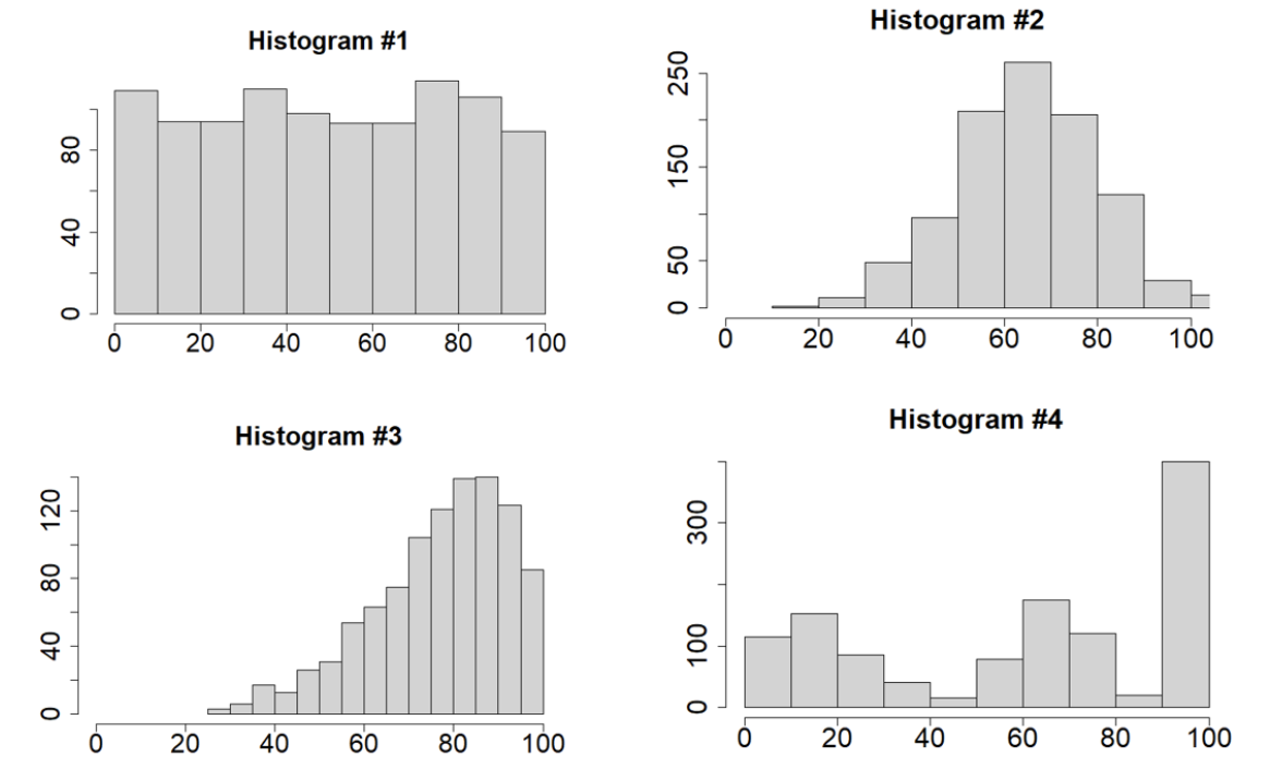
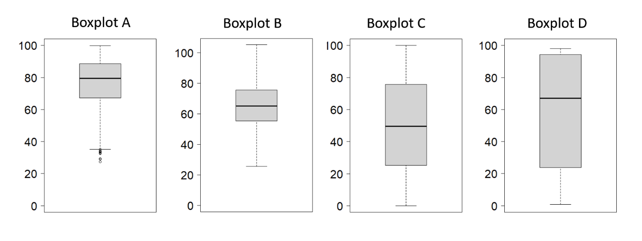
Question 1: Match each histogram to its corresponding boxplot:
- Histogram 1 corresponds to Boxplot
- Histogram 2 corresponds to Boxplot
- Histogram 3 corresponds to Boxplot
- Histogram 4 corresponds to Boxplot
Use the shape (skewness and symmetry), the center (mean/median), and the spread/range of the distributions displayed in the histograms to determine which boxplots share those characteristics. You may need to use process of elimination.
- C
- B
- A
- D
- Histogram 1 corresponds to Boxplot C. The histogram shows a roughly uniform or flat distribution with data is spread evenly between 0 and 100. Boxplot C reflects this with a very wide interquartile range (the box) and whiskers that extend across most of the range. The median is near 50, as expected for a symmetric distribution on [0, 100].
- Histogram 2 corresponds to Boxplot B. The histogram shows a symmetric, unimodal (bell-shaped) distribution centered near 65. Likewise, Boxplot B displays a symmetric distribution with the median line around 65 and whiskers of similar length.
- Histogram 3 corresponds to Boxplot A. The histogram is clearly left-skewed, with data concentrated between measurements of 80 to 90. The box in Boxplot A contains left skew because the median is closer to the third quartile (top of box) than the first quartile (bottom of box). Further, the bottom whisker extends further than the top whisker and there are several small-value outliers indicated, both consistent with left-skew.
- Histogram 4 corresponds to Boxplot D. The histogram is multi-modal, which boxplots are not usually effective at displaying. Measurements extend the full range from 0 to 100 which is consistent with the large variability (wide box) in Boxplot D.
Question 2: Imagine you are interested in the concentration of lead in the public drinking water system for two different cities (call them City A and City B). You collaborate with investigators in each city to obtain lead concentration measurements ($\mu$g/L) from a random sample of homes. The investigators sends you the following tables of summary statistics.
City A:
City B:
City A:
| Sample Mean | Sample Median | Sample Standard Deviation (S) |
|---|---|---|
| 7.3 | 4.9 | 5.87 |
| Minimum | Q1 | Q2 (Median) | Q3 | Maximum |
|---|---|---|---|---|
| 2.4 | 4.0 | 5.3 | 6.5 | 8.3 |
- Based on the available information, what is your best guess for the shape of the distribution of lead concentration measurements in each city? Your options are symmetric, left skewed or right skewed.
- Based on the summary tables, are you concerned about potential outliers or extreme observations in either set of data?
a) For City A, compare the sample mean and the sample median. If the mean is greater than the median, what does that suggest about the shape? For City B, compare the distances between the median (Q2) and the other quartiles (Q1, Q3), and between the median and the min/max values.
b) For City A, consider what a large standard deviation relative to the mean implies, especially when the data (lead concentration) cannot be negative. For City B, use the 1.5×IQR rule to check if the minimum or maximum values are outliers.
b) For City A, consider what a large standard deviation relative to the mean implies, especially when the data (lead concentration) cannot be negative. For City B, use the 1.5×IQR rule to check if the minimum or maximum values are outliers.
- City A: Right-skewed. City B: Symmetric.
- City A: The combination of right skew and large standard deviation relative to the mean suggests the potential for extreme measurments. City B: No, the minimum and maximum measurements are not outliers based on the 1.5xIQR rule.
a) Shape of Distribution:
- City A: The mean (7.3) is substantially greater than the median (4.9) given the scale of the measurements. This indicates that the distribution is likely right-skewed. Larger measurements are pulling the mean up, away from the center of the data (the median).
- City B: The distribution appears symmetric. We can check the distances from the center:
- Q2 to Q1: $5.3 - 4.0 = 1.3$
- Q2 to Q3: $6.5 - 5.3 = 1.2$ (very similar)
- Median to Min: $5.3 - 2.4 = 2.9$
- Median to Max: $8.3 - 5.3 = 3.0$ (very similar)
- City A: We should be concerned about potential outliers. The right-skewness (mean > median) suggests the potential for outliers. Furthermore, the sample standard deviation ($s=5.87$) is larger than the sample median ($\bar{x}=4.9$). Since lead measurements cannot be negative, a standard deviation this large relative to the center of the data indicates that there must be some large extreme values to create such a wide spread.
- City B: We can check for outliers using the 1.5×IQR rule. The Interquartile Range (IQR) is $Q3 - Q1 = 6.5 - 4.0 = 2.5$.
- Lower bound: $Q1 - 1.5 \times IQR = 4.0 - 1.5 \times 2.5 = 4.0 - 3.75 = 0.25$. The minimum value (2.4) is above this bound.
- Upper bound: $Q3 + 1.5 \times IQR = 6.5 + 1.5 \times 2.5 = 6.5 + 3.75 = 10.25$. The maximum value (8.3) is below this bound.
Question 3: A professor suspects that students in his statistics class do not sleep for eight hours per night on average. Ten students are randomly selected from the class and given journals to monitor the number of hours they sleep each night. The following data is observed, with the number of hours of sleep per night for each student averaged over a one-month monitoring period:
| Participant | Hours slept |
|---|---|
| 1 | 9.2 |
| 2 | 5.6 |
| 3 | 7.5 |
| 4 | 8.9 |
| 5 | 7.0 |
| 6 | 7.1 |
| 7 | 7.9 |
| 8 | 7.7 |
| 9 | 7.6 |
| 10 | 5.8 |
- Compute the sample mean $\bar{X}$ and sample standard deviation $s$ for the measurements. You can compute these quantities using software (e.g.,$R$) or by hand. Note that the formula for sample standard deviation is \[s=\sqrt{\frac{\sum (x_i - \bar{x})^2}{(n-1)}}\]
- State the null and alternative hypotheses (in symbols and words) for a one-sample t-test to test the hypothesis that students do not sleep an average of eight hours per night.
- Calculate the test statistic and state your conclusion for the hypothesis test at the $\alpha = 0.05$ level. The test statistic for a one-sample t-test is: \[ t = \frac{\bar{X}-\mu_0}{\frac{s}{\sqrt{n}}}\] and the critical values for a t-distribution with 9 degrees of freedom for a two-tailed $0.05$ test are $\pm2.262$.
- Suppose that, in truth, university students actually do sleep less than 8 hours per night on average. Given this, explain why we could observe data that results in a failure to reject the null hypothesis.
a) Calculate these directly from the 10 data points.
b) The null hypothesis is the statement of "no difference" from the proposed value (8 hours). The alternative is what the test is trying to find evidence for (i.e., the mean is not 8 hours).
c) Plug your values from part (a) into the t-statistic formula. Compare your calculated t-statistic to the given critical values.
d) What are properties of the true sleep times of students and and the specific sample collected by the professor that would limit our ability to detect the difference?
- Sample mean $\bar{x}=7.43$ and sample standard deviation $s \approx 1.15$.
- Let $\mu$ be the mean sleep time. $H_0: \mu = 8$ vs. $H_1: \mu \neq 8$. In words, the null hypothesis is that students sleep on average 8 hours per night, and the alternative is that they do not.
- The test statistic is $t \approx -1.57$. Since $-2.262 < -1.57 < 2.262$, we fail to reject the null hypothesis.
- Potential reasons for failing to detect a true difference include the small sample size (N=10), large variability in sleep times between students and/or a small difference in the true average sleep time and the null value of 8.
a) Sample Mean and Standard Deviation:
- Sample Mean ($\bar{X}$): $\frac{9.2+5.6+7.5+8.9+7.0+7.1+7.9+7.7+7.6+5.8}{10} = \frac{74.3}{10} = 7.43$
- Sample Standard Deviation ($s$): $s = \sqrt{\frac{\sum(x_i - \bar{X})^2}{n-1}} \approx 1.15$
- Symbols: $H_0: \mu = 8$; $H_1: \mu \neq 8$.
- Words: The null hypothesis ($H_0$) is that the true population mean sleep time for students is equal to 8 hours. The alternative hypothesis ($H_1$) is that the true population mean sleep time is not equal to 8 hours.
- Calculate the t-statistic: $$ t = \frac{\bar{X} - \mu_0}{s / \sqrt{n}} = \frac{7.43 - 8}{1.15 / \sqrt{10}} = \frac{-0.57}{1.15 / 3.162} = \frac{-0.57}{0.364} \approx -1.57 $$
- Conclusion: This one-sample t-test has N-1=9 degrees of freedom. We compare our calculated t-statistic (-1.57) to the critical values of $\pm 2.262$. Since our t-statistic is not more extreme than the critical values (it falls between -2.262 and +2.262), we fail to reject the null hypothesis. There is not enough statistical evidence to conclude that the average sleep time is different from 8 hours.
Question 4: The table below contains summary statistics a dataset comparing income by employment status.
| Steadily Employed? | Sample Size | Sample Mean | Sample Standard Deviation |
|---|---|---|---|
| Yes | 50 | 63.4 | 12.2 |
| No | 50 | 42.8 | 18.4 |
- Let $\mu_Y$ represent the mean income for those steadily employed and $\mu_N$ represent the mean income for those not steadily employed. Write the null and alternative hypotheses (using $\mu_Y$ and $\mu_N$) to test for a difference in mean income between those with and without steady employment in the past 12 months.
- Calculate the statistic for a two-sample t-test to perform the above hypothesis test, using the following formula: \[t=\frac{\bar{X}_Y - \bar{X}_N}{\sqrt{s_Y^2/n_Y+s_N^2/n_N}}\]
- State the decision of this hypothesis test at $\alpha=0.05$. For simplicity, you may compare the t-statistic to the $5\%$ critical values from a Normal Distribution ($\pm 1.96$).
a) The null hypothesis should state that there is no difference between the population means. The alternative should state that there is a difference.
b) Identify all the values from the table ($ \bar{X}_Y, \bar{X}_N, s_Y, s_N, n_Y, n_N $) and plug them into the formula.
c) If your calculated test statistic is more extreme (further from zero) than the critical value, you reject the null hypothesis.
b) Identify all the values from the table ($ \bar{X}_Y, \bar{X}_N, s_Y, s_N, n_Y, n_N $) and plug them into the formula.
c) If your calculated test statistic is more extreme (further from zero) than the critical value, you reject the null hypothesis.
- $H_0: \mu_Y = \mu_N$ vs. $H_1: \mu_Y \neq \mu_N$.
- $t \approx 6.60$
- Since $6.60 > 1.96$, we reject the null hypothesis. There is statistically significant evidence for a difference in mean income between the two groups.
a) Hypotheses: We are testing for any difference between the two groups, so it is a two-tailed test.
Since our observed t-statistic of 6.60 is much larger than the critical value of 1.96, it falls in the rejection region for the test. Therefore, we reject the null hypothesis. We have strong evidence to conclude that there is a statistically significant difference in mean income between those with steady employment and those without.
- Null Hypothesis ($H_0$): $\mu_Y = \mu_N$. (There is no difference in the population mean incomes).
- Alternative Hypothesis ($H_1$): $\mu_Y \neq \mu_N$. (There is a difference in the population mean incomes).
- $\bar{X}_Y = 63.4$, $s_Y = 12.2$, $n_Y = 50$
- $\bar{X}_N = 42.8$, $s_N = 18.4$, $n_N = 50$
Since our observed t-statistic of 6.60 is much larger than the critical value of 1.96, it falls in the rejection region for the test. Therefore, we reject the null hypothesis. We have strong evidence to conclude that there is a statistically significant difference in mean income between those with steady employment and those without.
Question 5: An investigator performs an experiment to determine the effectiveness of a water filtration device for removing lead from drinking water. The investigator first measures lead concentration (ppb=parts per billion) in 40 independent water samples. She then runs each water sample through the filter and re-measures lead concentration. The following data are obtained:
Would a two-sample t-test be appropriate to test for a difference in mean lead concentration in the pre- and post-filtering water samples? Explain your reasoning.
| Mean (ppb) | Standard Deviation (ppb) | |
|---|---|---|
| Pre-filtering | 13.44 | 3.21 |
| Post-filtering | 13.20 | 3.76 |
| Difference (Pre - Post) | -0.24 | 1.05 |
What assumptions are being made about the data when performing a two-sample t-test? Are they satisfied in this scenario? Consider the relationship between pre- and post-filtering measurements.
The two-sample t-test assumes independence between measurements. Because the same water samples are used for pre- and post-filtering, the set of pre- and post-filtering measurements are not independent. Therefore, a two-sample t-test is not the appropriate test to determine if the filtering is removing lead in this study design.
A two-sample t-test would not be appropriate. The two-sample t-test requires the measurements in the two groups being compared to be independent. Although the individual water samples are independent, the lead measurements in the pre- and post-filtering groups are not. The post-filtering measurement for each sample is dependent upon the initial pre-filtering measurement because they both come from the same water sample.
Because of the paired study design, the correct statistical test is a paired t-test. This test works by first calculating the difference in lead for each water sample (e.g., Pre - Post) and then performing a one-sample t-test on those differences to see if the mean difference is significantly different from zero.
Because of the paired study design, the correct statistical test is a paired t-test. This test works by first calculating the difference in lead for each water sample (e.g., Pre - Post) and then performing a one-sample t-test on those differences to see if the mean difference is significantly different from zero.